We will show how to use the QR2-code to perform single- and double-resonant (including the defect-induced double-resonant) Raman calculation in this tutorial with the typical two-dimensional material of graphene as an example. The involved input and output files can also be found in the GitHub project.
Firstly, let's create a directory named "Graphene" to perform all the following steps in the subdirectories created under this Graphene directory.
Quantum ESPRESSO calculation
- Self-consistent field calculation
- Phonon dynamical calculation
Create a subdirectory named "scf" and touch an input file (scf.in) in it as following for the self-consistent field calculation.
    &CONTROL
      calculation = 'scf'
      prefix = 'Gra'
      verbosity = 'high', disk_io = 'low'
      tstress = .true., tprnfor = .true.
      outdir = './tmp', pseudo_dir = '../pseudo'
    /
    &SYSTEM
      ibrav = 4
      celldm(1) = 4.6606698678, celldm(3) = 6.0819351481
      nat = 2, ntyp = 1
      ecutwfc = 120, ecutrho = 480
      occupations = 'smearing', smearing = 'mv', degauss = 0.01
      assume_isolated = '2D', vdw_corr = 'dft-d'
    /
    &ELECTRONS
      conv_thr = 1.d-13
    /
    ATOMIC_SPECIES
      C  12.010  C.upf
    ATOMIC_POSITIONS {crystal}
      C  0.3333333333  0.6666666667   0.0000000000
      C  0.6666666667  0.3333333333   0.0000000000
    K_POINTS {automatic}
      30  30  1  0  0  0
This will generate the ground-state charge density file saved in the "tmp" folder.
Creat a new subdirectory named "phonon" and the copy the "tmp" folder from the "scf" subdirectorty into it. The input file of "ph.in" for phonon calculation is as following
    phonon
    &inputph
      prefix = 'Gra'
      outdir = './tmp'
      nmix_ph = 20, tr2_ph = 1.0D-18
      verbosity = 'high', reduce_io = .true.
      fildyn = 'dyn', fildvscf = 'dvscf'
      ldisp = .true.
      nq1 = 15, nq2 = 15, nq3 = 1
    /
This will generate the lattice dynamical matrix files with names that start with "dyn" and also the deformation potential files contained in the "_ph0" folder.
EPW calculation
- Non self-consistent field calculation
- Wannierization calculation
Create a new subdirectory named "epw" and copy the "tmp" folder from the "scf" subdirectorty into it. To perform the epw calculation, it is necessary to first run a non self-consistent field calculation with the following input file of nscf.in
    &CONTROL
      calculation = 'nscf'
      prefix = 'Gra'
      verbosity = 'high', disk_io = 'low'
      tstress = .true., tprnfor = .true.
      outdir = './tmp', pseudo_dir = '../pseudo'
    /
    &SYSTEM
      ibrav = 4
      celldm(1) = 4.6606698678, celldm(3) = 6.0819351481
      nat = 2, ntyp = 1, nbnd = 13
      ecutwfc = 120, ecutrho = 480
      occupations = 'smearing', smearing = 'mv', degauss = 0.01
      assume_isolated = '2D', vdw_corr = 'dft-d'
    /
    &ELECTRONS
      conv_thr = 1.d-13
      diago_full_acc = .true.
      diago_thr_init = 1.d-13
    /
    ATOMIC_SPECIES
      C  12.010  C.upf
    ATOMIC_POSITIONS {crystal}
      C  0.3333333333  0.6666666667   0.0000000000
      C  0.6666666667  0.3333333333   0.0000000000
    K_POINTS {crystal}
      900
      0.00000000  0.00000000  0.00000000  1.111111e-03
      0.00000000  0.03333333  0.00000000  1.111111e-03
      0.00000000  0.06666667  0.00000000  1.111111e-03
      0.00000000  0.10000000  0.00000000  1.111111e-03
      0.00000000  0.13333333  0.00000000  1.111111e-03
      ...
    /
Compared to the scf calculation, the number of electronic bands is specifically given here as nbnd=13. These bands will be used to acquire the Wannier functions in the subsequent wannierization calculation. Note also that the k-points are given in individual coordinates rather than in the grid form, and it can be generated with a script called "kmesh.pl" in the "external/wannier90/utility/" directory of QE package.
In this epw subdirectory, touch a file named "epw.in" as the wannierization calculating input file. It is writen as following
    epw
    &inputepw
      prefix = 'Gra'
      outdir = './tmp', dvscf_dir = './save'
      system_2d = 'dipole_sp'
      asr_typ = 'crystal', vme = 'dipole'

      nbndsub = 5
      ep_coupling = .true., elph = .true.
      use_ws = .true., num_iter = 400

      dis_froz_min = -25, dis_froz_max = -1

      proj(1) = 'f=0.3333333333,0.6666666667,0.0000000000:sp2;pz'
      proj(2) = 'f=0.6666666667,0.3333333333,0.0000000000:pz'

      fsthick = 3, eps_acustic = 5
      degaussw = 0.005, degaussq = 0.01

      wdata(1) = 'dis_mix_ratio = 0.7'
      wdata(2) = 'dis_num_iter = 400'
      wdata(3) = 'conv_window = 3'
      wdata(4) = 'trial_step = 1.0'
      wdata(5) = 'guiding_centres=.true.'

      epwwrite = .true., epwread = .false.
      wannierize = .true., wannier_plot= .true.

      nk1 = 30, nk2 = 30, nk3 = 1
      nq1 = 15, nq2 = 15, nq3 = 1
      nkf1 = 3, nkf2 = 3, nkf3 = 1
      nqf1 = 3, nqf2 = 3, nqf3 = 1
    /
After this calculation, we will get a couple of files with extension of ".cube" each of which is one Wannier-function visuallization data and can be opened by the VESTA application. Besides, we can also find the crystal.fmt, dmedata.fmt, epwdata.fmt, Gra.ukk and Gra.epmatwp (in tmp folder) files which will be used to run the subsequent Raman calculation.
Single resonant Raman
- Raman intensity calculation
- Raman spectrum plotting
Create a new subdirectory named "single-raman/1.71eV" and the copy the crystal.fmt, dmedata.fmt, epwdata.fmt, Gra.ukk and epw.in files from the "epw" subdirectorty into "1.71eV" (you can also creat subdirectory, such as "1.96eV", for other laser energy calculation). Modify the epw.in file as following and rename it as "raman.in"
    epw
    &inputepw
      outdir = '../../epw/tmp', dvscf_dir = '../../epw/save'
      ...
      epwwrite = .false., epwread = .true.
      wannierize = .false., wannier_plot= .false.

      nk1 = 30, nk2 = 30, nk3 = 1
      nq1 = 15, nq2 = 15, nq3 = 1
      nkf1 = 100, nkf2 = 100, nkf3 = 1
      nqf1 = 1, nqf2 = 1, nqf3 = 1

      Raman_type = 'single', lhoph = .false.
      Elaser = 1.71, Egamma = 0.3
      reson_lim = .true., reson_thr = 1
      lBE = .false., temphon = 300
      prtdipole = .true., prtRaman = .true.
      polar = 'all', filraman = 'qraman'
      ei = (1.d0,0.d0), (0.d0,0.d0), (0.d0,0.d0)
      es = (1.d0,0.d0), (0.d0,0.d0), (0.d0,0.d0)
      Cq = 0.d0, 0.d0, 0.d0, 1.d0, 0.d0, 0.d0, 0.d0
      ltensor = .false., qtensor_start = 1, qtensor_end = 1
    /
In the above, we only show the changed part of epw.in file. epwread=.true. indicates that we are actually perform a restaring calculation of epw based on the Wannier-basis that we get in the wannierization calculation. The parameters in the bottom panel of raman.in are not present in the original EPW code, and they are specific to the QR2 code for resonant Raman calculation. Raman_type = 'single' specifies the single resonant Raman, and Elaser = 1.71 indicates the incident laser energy. For polar = 'all', we will finally get the Raman intensity files of qraman-xx, qraman-yy, qraman-xy, qraman-yx, qraman-ll, qraman-rr, qraman-lr and qraman-rl which are in different geometric configuration. "xx" represents the incident and scattered light propogating in z direction and both polarized in x direction. "l (r)" means left (right) circularly polarized light.
In the above calculation, we get the Raman intensity data with which we can only plot the Dirac peaks rather than the Raman band with finite bandwidth. This post-processing implementation broadens the Raman peak with a Lotentz function parameter Lgamma. Create a new subdirectory of "xx" under "single-raman/1.71eV" to tackle with the qraman-xx data. The standard input file of raman_pp.in looks like the following
&PLOT
dir_raman = '../qraman-xx'
Raman_type = 'single', lhoph = .false.
lRay_sca = .false., Ray_thr = 5
Rs_min = -2000, Rs_max = 2000, Rs_inc = 0.1
Lgamma = 10
/
&ANALYSIS
lRaman_modes = .false.
nphonon_modes = 6
nRaman_modes = 1
Raman_modes(1) = 50.d0
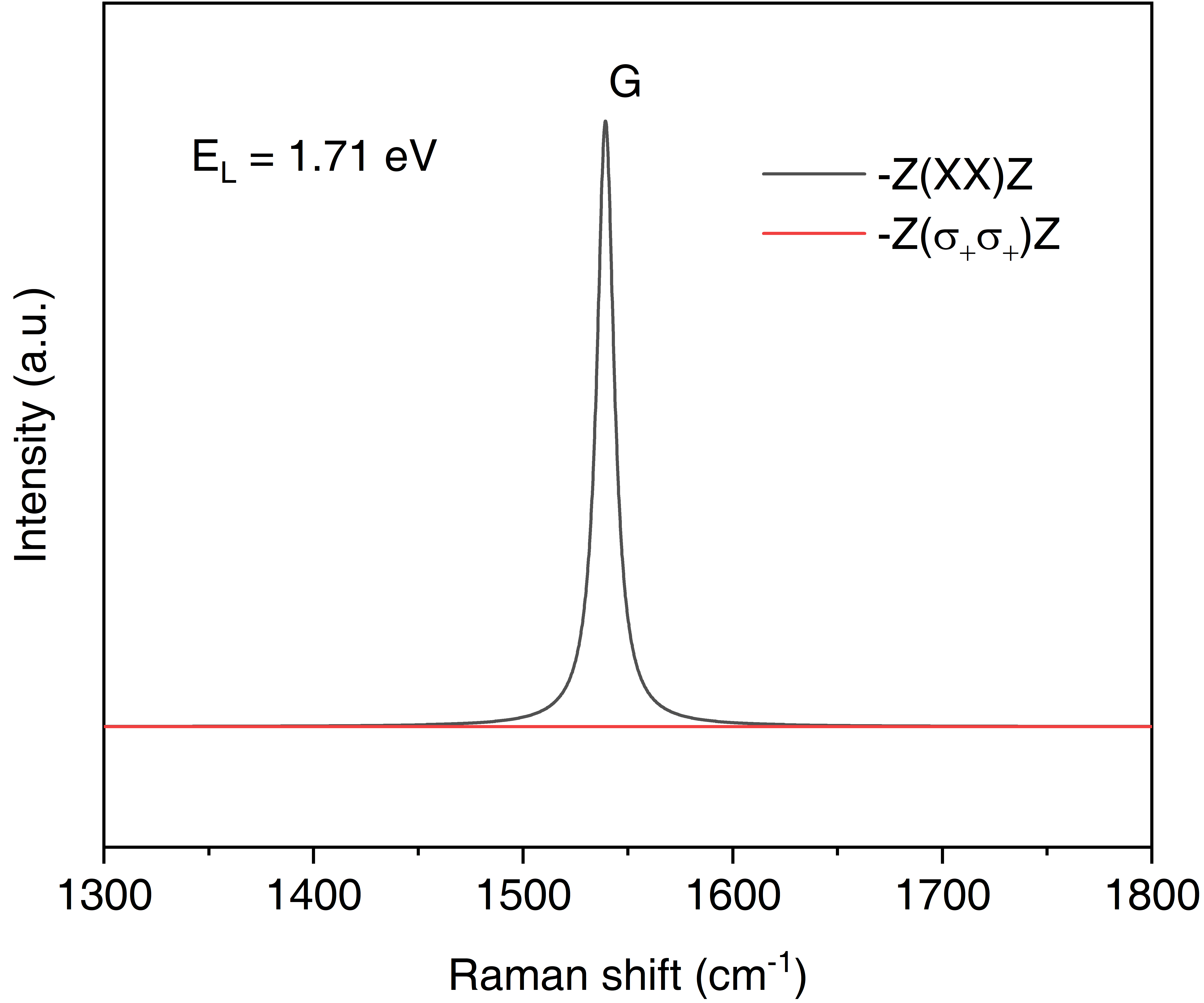
/This will generate a file of "Raman.dat" with which we can plot the Raman spectrum. We can also create another subdirectory of "ll" under "single-raman/1.71eV" to tackle with the qraman-ll data and get the circularly polarized Raman spectrum. The final single resonant Raman plot of graphene are as shown in following figures. Note that in single resonant Raman case, the phonon modes originate from \(\Gamma\) point and it is usually quite easy to assign the Raman mode by inspection, so the lRaman_modes can be always set to .false.
Double resonant Raman
- Raman intensity calculation
- Raman spectrum plotting
- Raman mode analysis
Analogously to the single Raman case, create a new subdirectory named "double-raman/1.71eV" and copy the crystal.fmt, dmedata.fmt, epwdata.fmt, Gra.ukk and epw.in files from the "epw" subdirectorty into it. The raman.in input file is as follows
    epw
    &inputepw
      outdir = '../../epw/tmp', dvscf_dir = '../../epw/save'
      ...
      epwwrite = .false., epwread = .true.
      wannierize = .false., wannier_plot= .false.

      nk1 = 30, nk2 = 30, nk3 = 1
      nq1 = 15, nq2 = 15, nq3 = 1
      nkf1 = 100, nkf2 = 100, nkf3 = 1
      nqf1 = 100, nqf2 = 100, nqf3 = 1

      Raman_type = 'double', lhoph = .true.
      Elaser = 1.71, Egamma = 0.3
      reson_lim = .true., reson_thr = 1
      lBE = .false., temphon = 300
      prtdipole = .true., prtRaman = .true.
      polar = 'custom', filraman = 'qraman-xx'
      ei = (1.d0,0.d0), (0.d0,0.d0), (0.d0,0.d0)
      es = (1.d0,0.d0), (0.d0,0.d0), (0.d0,0.d0)
      Cq = 0.d0, 0.d0, 0.d0, 1.d0, 0.d0, 0.d0, 0.d0
      ltensor = .false., qtensor_start = 1, qtensor_end = 1
    /
Since the double resonant Raman involes the phonon modes throughout the Brillouin zone, the fine q-point is specified in a dense grid of 100\(\times\)100. Raman_type is set to "double" to perform double resonant Raman calculation. We also consider the hole-phonon scattering in Raman scattering process by setting lhoph = .true.. We explicitly set the -Z(XX)Z geometric configuration in parameters "ei" and "es" by choosing polar = 'custom'. After the calculation, the Raman intensity data will be printed in a file named "qraman-xx".
Create a new subdirectory of "xx" under "double-raman/1.71eV" to tackle with the qraman-xx data and the raman_pp.in file is given as follows
&PLOT
dir_raman = '../qraman-xx'
Raman_type = 'double', lhoph = .true.
lRay_sca = .false., Ray_thr = 5
Rs_min = -4000, Rs_max = 4000, Rs_inc = 0.1
Lgamma = 10
/
&ANALYSIS
lRaman_modes = .false.
nphonon_modes = 6
nRaman_modes = 1
Raman_modes(1) = 50.d0
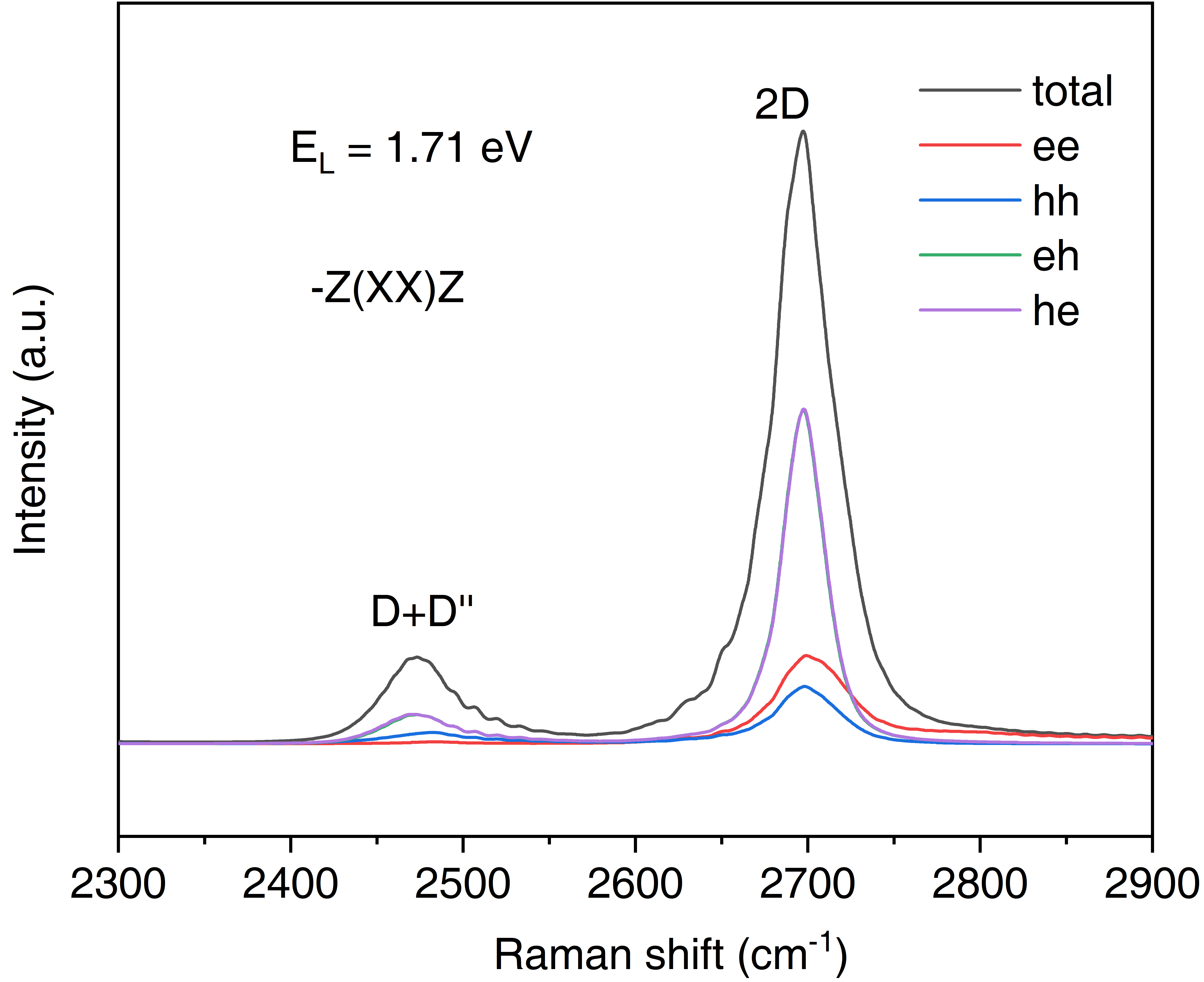
/This will generate a file of "Raman.dat" with which we can plot the Raman spectrum. In the "Raman.dat", not only generate the total Raman intensity Itot, but also the component of Iee, Ihh, Ieh and Ihe, each with four scenarios of phonon combination (pp, mm, pm, mp). The Raman spectrum plot is shown below where two double resonant mode of D+D'' and 2D are obvious at 2473.3 cm-1 and 2697.3 cm-1, respectively. Due to the special band structure of graphene, the Raman intensity of eh and he component is significantly stronger than the ee and hh.
Then setting lRaman_modes = .true. in raman_pp.in as below allows us to perform the Raman mode analysis, i.e., the Raman assignment. Here we analyze the D+D'' and 2D by inputting their corresponding Raman shift. For each Raman mode, 6 phonon-pairs in descending order in terms of contribution to the total Raman intensity will be presented in the output files.
&PLOT
dir_raman = '../qraman-xx'
Raman_type = 'double', lhoph = .true.
lRay_sca = .false., Ray_thr = 5
Rs_min = -4000, Rs_max = 4000, Rs_inc = 0.1
Lgamma = 10
/
&ANALYSIS
lRaman_modes = .true.
nphonon_modes = 6
nRaman_modes = 2
Raman_modes(1) = 2473.3d0
Raman_modes(2) = 2697.3d0
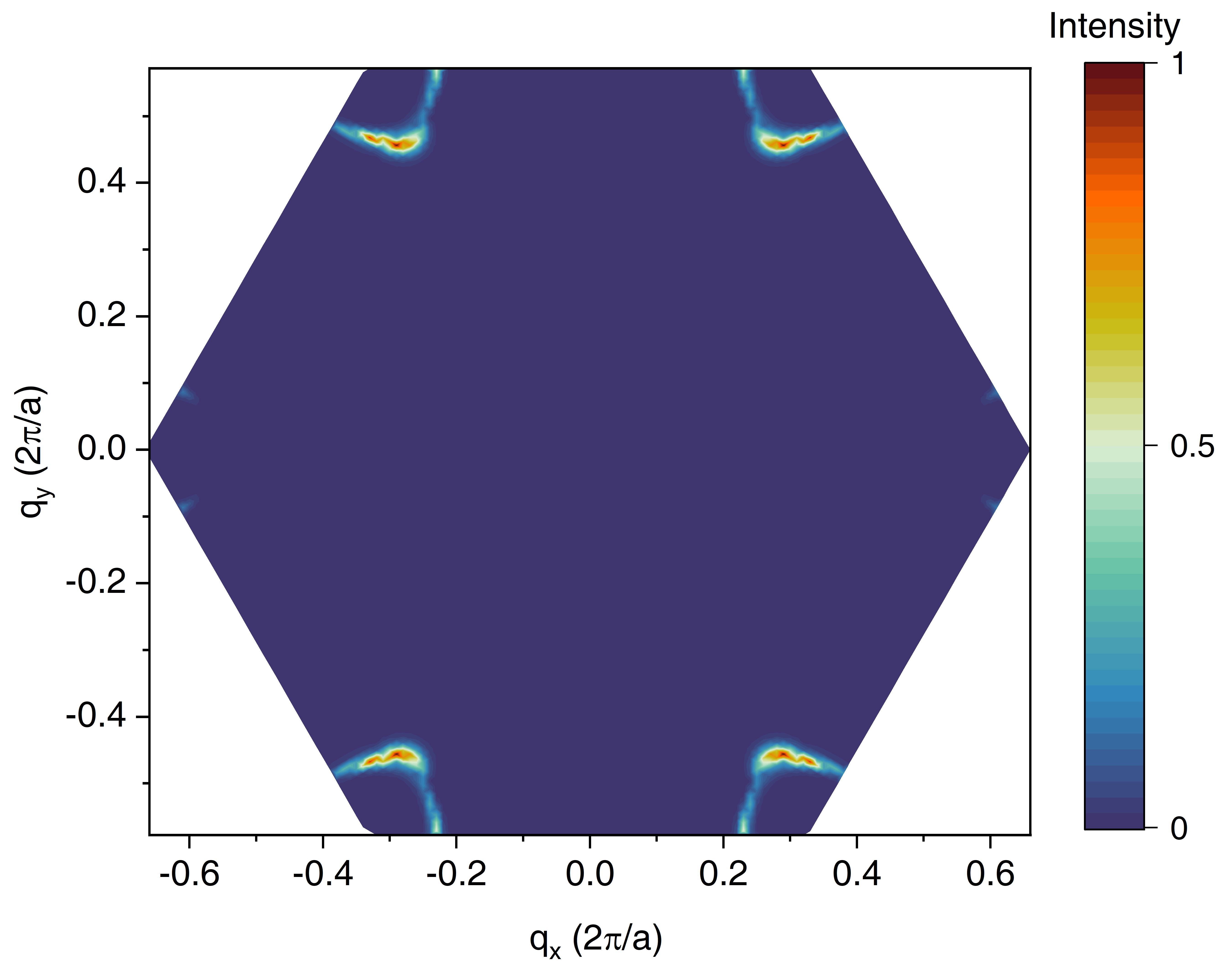
/In the output file of raman_pp.out, the phonon mode (branch) combinations that contribute significantly to the total Raman intensity and their correspoding weight are given. Moreover, you can visualize the Raman intensity of each q-point in the Brillouin zone with the help of output files Raman_mode01 and Raman_mode02. The q-resolved Raman intensity of 2D Raman mode is shown below and it can be seen that the q points that decide the 2D Raman mode mainly reside around the K (K') point.